Seamless heightmaps

This chapter describes how to use the gradient noise functions and the blueprint from the previous chapters to generate seamless heightmaps from triangular patches. If you have not already, I strongly suggest to at least read the notes on the blueprint first.

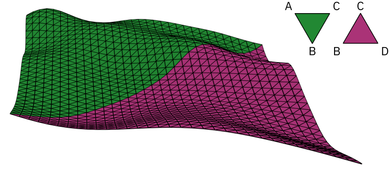
The idea behind the heightmaps is simple: we assign one noise function to each top level vertex of the blueprint. For all other vertices we interpolate between these noise functions – just as we have interpolated between vertex colors in the previous chapter. We then use the interpolated values as y-coordinates (height) of the vertices.

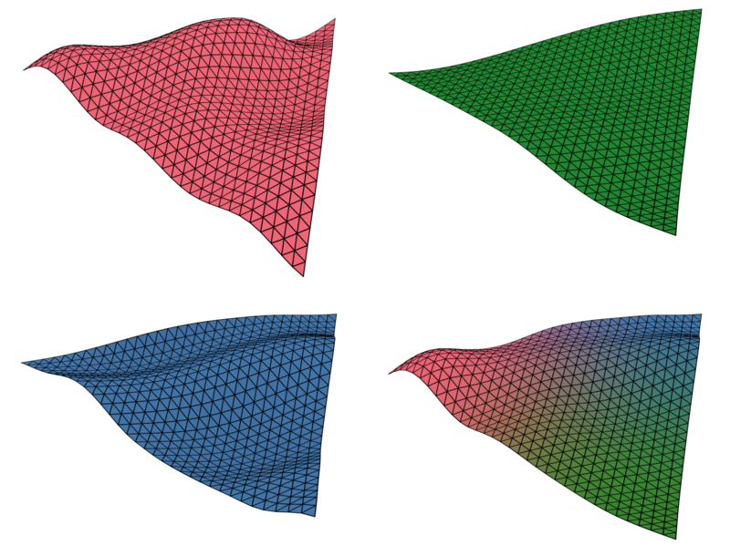
The green patch shown in the example above is derived from three noise functions A, B, and C, which are shown in the following figure in red, green, and blue respectively. Interpolating between the three functions results in the final patch shown in the lower right:

In order to generate multiple patches that together form a seamless heightmap, we have to pay special attention to the mapping between the coordinates of the blueprint and the coordinates of the noise functions.

If we furthermore want to use smooth shading for the generated terrain, we also need to take a closer look at the surface normals of the generated patches. Getting the surface normals right is also important for another reason: they will serve as basis for geometry effects used in the next chapters.

Coordinate mapping

When we assign a noise function to a top-level vertex of the blueprint, that function needs to cover more than the area of that single patch of terrain. Since we will use the same function to generate the neighboring patches, it has to cover an entire hexagon with side length one.

The noise functions used by Layercake are defined for the unit cube. Thus, in order to provide the required coverage, we need to scale and translate them accordingly (we are of course transforming the input coordinates and do not modify functions themselves). The following figure shows the setup we are going for. It is a top-down view on the xz-plane where the colored rectangles indicate the domains of the three noise functions.

So far we have ignored that the blueprint always points into the same direction. If we want to piece together two patches, we will have to rotate one of the two. For example, we can generate a second patch where we flip the assignment of the blue and red noise functions and rotate the patch by 60 degrees (clock-wise):

It is easy to see that this will not result in a seamless terrain: the mappings of the noise functions do not align.

There are two ways we could solve this. We could either create a second blueprint that faces in the opposite direction such that no rotation is required. Or we could apply the inverse rotation to the input of the noise functions.

I have decided for the second approach, since it can be implemented in a few lines of code and does not require other parts of the code base to make distinction between two different blueprints. The rotated mapping looks like this:

If we now generate two patches with matching noise functions, one using the rotated mapping, we can combine the two patches such that everything is aligned:

Note that there is no need for further transformations of the coordinate systems. To build larger terrains, we can extend the example above by alternating between patches with non-rotated mappings and patches with mappings rotated by 60 degrees.

Surface normals

Using the coordinate transformations discussed in the previous section, we can generate patches that result in a seamless heightmap when combined. The following image shows a flat shaded rendering of the two patches from the beginning of this chapter (using Blender). It uses a material that maps the surface normals of the geometry to RGB color values (similar to a normal map):

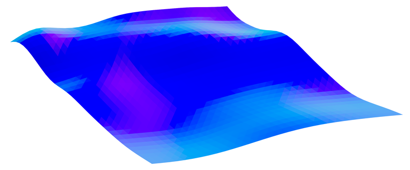
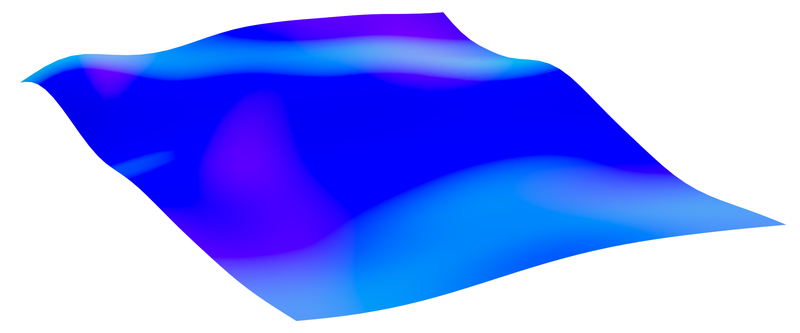
There is nothing wrong with this rendering. In particular, there is nothing giving away that the prism consists of two triangular patches that were generated independently from each other. However, things change when we switch to smooth-shading. There are subtle but clear discontinuities in the color (surface normals) along the boundary between the two patches:

This is not surprising given how Blender (and other 3D software) derives surface normals for smooth shading. When rendering a pixel of a face, Blender derives the surface normal for that pixel by interpolating between the vertex normals of the face. Since we have not specified any vertex normals, Blender derives those by looking at the neighboring vertices. This neighborhood is not fully known for vertices along the edges of a patch. Thus, we end up with different normals along the patch boundaries.

When working with a software such as Blender, we can of course fix this easily by merging the two patches into a single structure. However, this is not a good solution for applications where we might want to generate or modify the terrain on the fly.

The keep the patch generation independent from its neighbors, we need to compute the vertex normals in a way that does not require looking at the neighboring vertices.

Conceptually, this is very simple. The heightmaps are basically 3D plots of our noise functions. And just as you can derive the orthogonal of a one-dimensional function from its slope, you can derive the normal of a higher-dimensional function from its gradient. So all we have to do is to determine the gradients at the vertex positions.

You might be wondering whether we already have all the information we need. After all, we implemented our very own gradient noise functions. Unfortunately, we cannot just look the gradients up: we only know the few gradients we picked for the grid points and all other are interpolated.

But we do know the math behind the noise functions. So we could try to compute the derivative. To put it short, while I did manage to compute the derivative using a library for symbolic mathematics, the resulting code is not something I want anyone to maintain. Fortunately, there is no need to be mathematically accurate. As long as it looks good, an approximation will be sufficient.

We can approximate the gradient by sampling the the function three times at (x, y, z), (x + ε, y, z), and (x, y, z + ε) for some small value of ε. Since we are only sampling 2D coordinates, there is no need to compute the change along the y-axis. Deriving the normal is then straight-forward. As we will discuss in the implementation section we only have to be careful with being consistent in our inaccuracies.

Loading these approximated normals in Blender, we get the following result, which is very similar to blenders generated surface normals, but without the discontinuities:

If you are wondering whether smooth-shading is worth the trouble, consider that computing the vertex normals by ourselves opens up further possibilities. In particular, we will use the normals in the following chapters to deform the generated geometry.

Implementation

If you have not already, I recommend reading the general notes on the source code and the included math package first. In particular, if you are not familiar with Java.

You can find the implementation of the heightmap generation in HeightmapGenerator.java – a single class with less than 200 lines of code. A short example generating the two patches used throughout this chapter is given in Heightmaps.java.

The generator

A single instances of an HeightmapGenerator can be used to generate multiple patches. The idea is to reuse temporary buffers whenever possible – this will become more relevant in the following chapters. Multi-threading can be achieved by using one generator instance per worker-thread. The generators themselves are not thread-safe.

For the sake of simplicity, this generator implementation does not generate meshes in a GPU friendly format. Instead, it outputs strings in the Wavefront object format. This should allow for importing the meshes into most 3D modeling software.

Constants

The generator initializes the rotation matrices for the coordinate mapping once for all generator instances. Layercake uses a right-handed coordinate system with y pointing up and the blueprint lies on the xz-plane. Thus, we rotate around the y-axis.

private static final Mat3f ROTATION_60_DEG = Mat3f.yRotation(-Math.PI / 3d);
private static final Mat3f ROTATION_M60_DEG = Mat3f.yRotation(Math.PI / 3d);
private static final Mat3f ROTATION_NONE = Mat3f.identity();

Similarly, the positions of the top-level vertices are looked up once during initialization. They are named ORIGIN_X etc., since one can think of the transformation of the coordinates as specifying three coordinate systems centered at these vertices.

private static final Vec3f ORIGIN_X, ORIGIN_Y, ORIGIN_Z;

static {
    Cell root = BLUEPRINT.root();
    Vec3fList positions = BLUEPRINT.positions();
    ORIGIN_X = positions.get(root.vertexX, new Vec3f());
    ORIGIN_Y = positions.get(root.vertexY, new Vec3f());
    ORIGIN_Z = positions.get(root.vertexZ, new Vec3f());
}

There are three constant relevant for the computation of the surface normals. EPSILON is used to approximate the gradient. In theory, one should choose an arbitrary small value for ε. In practice, we have to consider the limited precision of 32Bit floating point values.

private static final float EPSILON = 0.001f;
private static final float SAMPLE_HEIGHT = 0.5f;
private static final float NORMAL_HEIGHT = 5f;

The SAMPLING_HEIGHT is a scaling factor applied to the height of the terrain. The chosen value flattens the terrain. As a consequence, the normals need to be adjusted as well. This is where NORMAL_HEIGHT comes into play. Please note that this value was not derived using some formula. Instead, I simply played around with values until the results matched the normals computed by Blender.

Initialization

The initialization code inside the generate(...) method is straight-forward. Note that instead of keeping a flag around whether to rotate the coordinates, the code simply sets the generator’s rotation matrices to the identity matrix in case no rotation is required.

/**
 * Generates a new heightmap in Wavefront Object format using the given
 * noise functions.
 *
 * @param x      the noise function for vertex x
 * @param y      the noise function for vertex y
 * @param z      the noise function for vertex z
 * @param rotate whether to rotate coordinates by 60 degrees
 * @return the heightmap in Wavefront Object format
 */
public String generate(Noise x, Noise y, Noise z, boolean rotate) {
    this.noiseX = x;
    this.noiseY = y;
    this.noiseZ = z;
    this.rotation = rotate ? ROTATION_60_DEG : ROTATION_NONE;
    this.inverseRotation = rotate ? ROTATION_M60_DEG : ROTATION_NONE;
    sampleVertices();
    return writeWavefront();
}

Sampling

The sampling of a single noise function is implemented in the sample(...) method. It includes the computation of the partial gradient:

/**
 * Samples the given noise function at the given position and approximates
 * the partial gradient (x- and z- axis only).
 *
 * @param noise    the noise function
 * @param origin   the origin of the noise function in the source
 *                 coordinate system
 * @param position the position to sample
 * @param gradient the partial gradient
 * @return the sample of the given position
 */
private float sample(Noise noise, Vec3f origin, Vec3f position,
                     Vec3f gradient) {
    // ...
}

The method first transforms the given blueprint coordinates into the coordinates of the noise function centered around the given origin:

// Translate the given position into the coordinate system with the
// given origin and map from [-1, 1] to [-0.5, 0.5].
Vec3f vertex = new Vec3f();
vertex.x = (position.x - origin.x) * 0.5f;
vertex.z = (position.z - origin.z) * 0.5f;

// Rotate coordinates around the origin.
vertex = rotation.mul(vertex, vertex);

// Translate again to map from [-0.5, 0.5] to [0, 1].
vertex.x += 0.5f;
vertex.z += 0.5f;

Next, three samples are take to determine the value itself as well as the gradient. Please note that ε is added after rotating the coordinates. This ensures that any inaccuracies due to the use of ε are independent of the rotation matrix. It also allows us to get away with relatively large values of ε so that we do not have to worry about rounding errors:

// We need three samples to approximate the gradient at the given
// position (only along the x- and z-axis). EPSILON is added after the
// rotation to ensure that we always sample the same three points
// regardless of orientation (we cannot choose an arbitrarily small
// value for EPSILON due to the limited precision of 32Bit floats).
float sample = noise.sample(vertex.x, 0f, vertex.z);
float sampleDx = noise.sample(vertex.x + EPSILON, 0f, vertex.z);
float sampleDz = noise.sample(vertex.x, 0f, vertex.z + EPSILON);

gradient.x = (sampleDx - sample) / EPSILON;
gradient.z = (sampleDz - sample) / EPSILON;

There is just one problem with this approach. If we rotate the coordinate but not the ε offsets, the resulting gradient points into the wrong direction. We can fix this by applying the inverse rotation to the gradient before returning the sample:

// Since we did not include EPSILON in the rotation, we need to
// adjust the orientation of the gradient.
inverseRotation.mul(gradient, gradient);
return sample;

Interpolation

The interpolation between the three noise function is implemented in sampleVertices(). This comes down to combining the results of the three calls to sample(...) using the respective influence weights:

for (int i = 0; i < positions.size(); i++) {
    normal.set(0f, NORMAL_HEIGHT, 0f);
    position = positions.get(i, position);
    weight = weights.get(i, weight);

    float sample = weight.x * sample(noiseX, position, ORIGIN_X, gradient);
    normal.add(gradient.scl(weight.x));

    sample += weight.y * sample(noiseY, position, ORIGIN_Y, gradient);
    normal.add(gradient.scl(weight.y));

    sample += weight.z * sample(noiseZ, position, ORIGIN_Z, gradient);
    normal.add(gradient.scl(weight.z));

    vertices.set(i, position.x, sample * SAMPLE_HEIGHT, position.z);
    normals.set(i, normal.norm());
}

Note how we fill in NORMAL_HEIGHT for the missing y-value of the gradient.

That’s it. To get more familiar with the code I recommend starting with the example provided in Heightmaps.java.