The blueprint

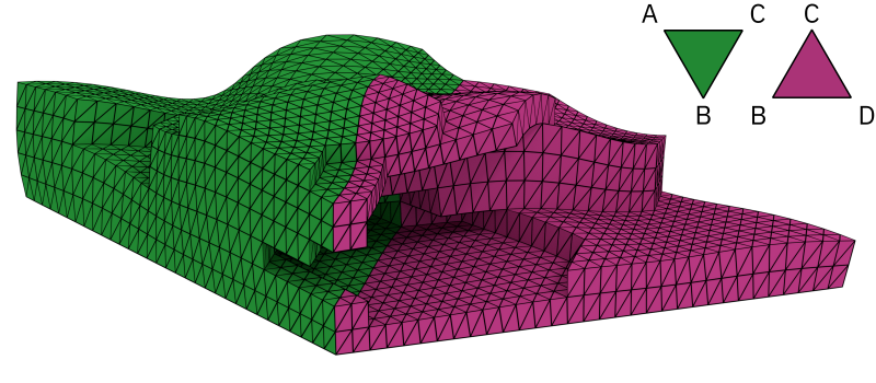
The blueprint is a small and simple helper construction that we will use as basis to build triangular patches of terrain. For example, the two patches (A, B C) and (C, B, D) in the figure below are constructed from the same blueprint but with different attributes/parameters for vertices A and D:

The blueprint is at its core a multiple times subdivided, equilateral triangle. It is a static construction that is the same for all patches.

In addition to vertex positions, the blueprint also contains information on how to blend between parameter sets. In the example above, it is used to ensure that the edges (B, C) and (C, B) match perfectly. The information encoded in the blueprint can be summarized as:

• Vertex positions: the positions of all vertices on the xz-plane (Layercake uses a right-handed coordinate system where y is up).
• Weights for blending: the blueprint provides influence weights for blending between vertex attributes for the three vertices of the top level triangle.
• The subdivision graph: the blueprint allows for easy navigation of the subdivided triangle, e.g., looking up parent, child, and sibling triangles.

The computations of the vertex positions contains no surprises, but there are some details to consider when choosing the blending weights. Maintaining the subdivision graph is for the most part an implementation detail that we will cover in the corresponding section.

Vertex positions

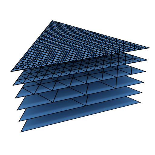
The top level triangle is always equilateral with side length one. It is centered around the origin and points in the z-direction. At the third subdivision level the blueprint looks like this:

The patches shown at the top of this page use a blueprint with five subdivisions. They also show how one can utilize the different subdivision levels: using a lower level (larger triangles) to decide which parts of the terrain are solid helps achieving a low-poly look.

Weights for blending

Given a set of attributes defined for the three vertices of the top level triangle, the influence weights define how to interpolate between those attributes for all other vertices. Examples of attributes are vertex colors, y-positions, or the result of a texture look up.

It is not enough for the weights to provide smooth interpolation for a single patch. They also need to satisfy the following requirements:

1. The interpolated values along the edges of the top level triangle must be independent from the attributes of the opposite vertex, e.g., in a triangle (A, B, C), the weights for C must be zero for all points along the edge (A, B).
2. The weights must be chosen in a way that the triangular base does not become visible when combining multiple patches.

As we will see, weights satisfying the first requirement do not automatically satisfy the second.

Barycentric coordinates

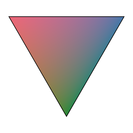
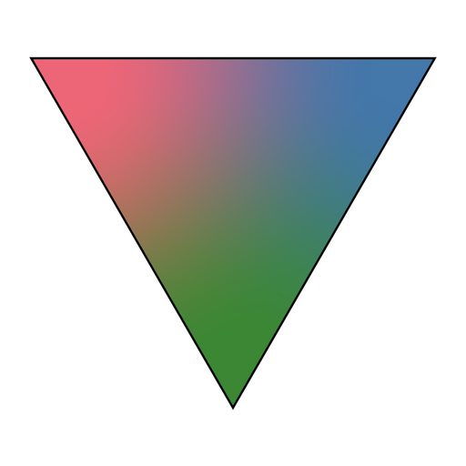
Tutorials for graphics APIs such as OpenGL often start with drawing a colorful triangle such as the one shown below. You specify two attributes per vertex – its position and color – and your graphics hardware does the rest. In particular, we end up with a smooth interpolation between vertex colors that seem to satisfy the requirements listed above. So why not just compute weights using the same blending function?

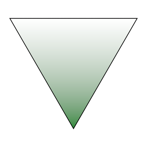
At least in the case of OpenGL this blending function is based on barycentric coordinates. And while it does look great for a single triangle, it does not satisfy the second requirement. The reason for this becomes apparent if we color only the bottom vertex. Its blend factor decreases linearly along the angle bisector:

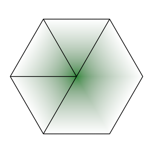
If we construct a hexagon consisting of six of these triangles, we can clearly see the where one triangle ends and the next begins:

To prevent artifacts like this we will need to implement another blending function. Something close to a radial gradient might work which hints at a distance-based approach using Euclidean coordinates:

Euclidean coordinates

We have already implemented a distance-based blend function using Euclidean coordinates in the first chapter discussing gradient noise. There we interpolated between a set of linear functions, here we compute weights to blend between arbitrary vertex attributes.

For the values along the edges of the top level triangle we could use the same interpolation method as for the one-dimensional case of the gradient noise. However, determining the weights for the inner vertices is, while similar, not the exact same problem as the two-dimensional case. The triangular grid does not allow for the same two-step approach as the rectangular one (blending one axis at a time).

What we can reuse is the idea of using the smoothed inverse distance. Let’s start with that.

The blueprint is an equilateral triangle with side-length one. To ensure that the weights along its edges are independent of the opposite vertex the weight for that vertex must be zero for all points with a distance equal or larger than the height h = 0.5 · √3 of the blueprint.

This can be seen in the following figure. The outer circle is the unit circle around the center vertex which includes its opposing edges. The inner circle has radius h and only touches those edges. In other words, if we limit the influence of the center vertex to the inner circle, we satisfy the first requirement listed above:

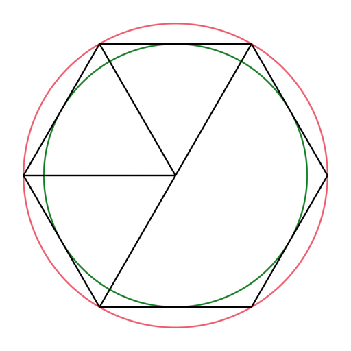
To do so we have to scale and clamp the distance d before we can smooth it. Instead of using smooth(1 - d) as for the gradient noise, we have to use smooth(max(0, 1 - d / h)) as weight.

There is just one minor flaw: repeating the step for the other two vertices will give us three influence weights, but the sum of these weights is not constant across the blueprint. The fix for this is easy. We simply normalize the weights such that they always add up to one.

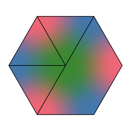
Using the generated weights to blend between color attributes we get the following result (same colors as before):

Looking at the hexagon, we can still see hints of the underlying triangular grid. In particular, the green center is not a perfect radial gradient. However, the result should be smooth enough for our purpose:

Implementation

If you have not already, I recommend reading the general notes on the source code and the included math package first. In particular, if you are not familiar with Java.

The blueprint is implemented as singleton in Blueprint.java. Vertex positions, relations, and weights are computed only once during initialization:

private Blueprint() {
    // Build tree/heap structure
    buildHeap();
    connectSibling();
    // Determine vertex ids
    assignVertexIds();
    // Determine vertex positions and weights
    initPositions();
    initWeights();
}

For this reason, little effort went into polishing or optimizing those methods. However, the code should be straight-forward to read once you understand the underlying data structure: under the hood, the blueprint is a complete and fully connected quad-tree that is furthermore stored as heap.

The root node or Cell of this tree is the top level triangle of the blueprint (the one with side length one). Cell instances keep references to their parents, their four children, and to their siblings. Furthermore, they know their orientation, the integer ids of their three vertices, and their own integer id (position in the heap). Vertex positions and weights are stored separately in two Vec3fList instances.

This setup allows to traverse the blueprint both recursively and level by level. For recursive traversal, one can start with the root node returned by Blueprint#root() and follow its references.

To traverse the blueprint level by level (or to iterator over a single level), one can work with the methods Blueprint#cellCount(int subdivisions) and Blueprint#cell(int id). The first method returns the absolute number of cells of a quad-tree with the given number of subdivisions which also happens to be the heap index of the first Cell at the next subdivision level. The second method simply returns the Cell with the given id:

for (int level = 0; level <= Blueprint.SUBDIVISIONS; level++) {
    int firstOnLevel = Blueprint.cellCount(level - 1);
    int firstOnNextLevel = Blueprint.cellCount(level);
    for (int id = firstOnLevel; id < firstOnNextLevel; id++) {
        Cell cell = BLUEPRINT.cell(id);
        // ...
    }
}

An example that traverses the blueprint this way can be found in BlueprintLevels.java. This class generates a simple 3D mesh of the blueprint in the Wavefront object format:

Given that the blueprint is a helper construction to be used by other code, I recommend reading the next chapter first before diving deeper into its implementation. It will provide a more interesting examples of its usage.