Gradient noise

This chapter describes the implementation of a simple gradient noise function that is almost identical to the classical Perlin noise. If you are already familiar with Perlin noise or Simplex noise, feel free to skip this chapter.

Overview

While the idea behind gradient noise is simple, it might be at first difficult to see how it results in random clouds. For this reason, we will first take a look at the one- and two-dimensional cases, before jumping into the generation of noise volumes.

The approach however is always the same: We first partition the domain (the input range) of the noise function into a regular grid. For each vertex of the grid we then pick a random gradient and a random offset. These two values together with the vertex coordinates define a linear function. To sample the noise function we first lookup the cell enclosing the point and then interpolate between the linear functions associated with its vertices.

Wobbly lines (1D noise)

The output of a one-dimensional gradient noise function is a curve that already displays the properties of the random clouds we will generate later on: its slope appears to change randomly but the transition is always smooth. In particular, there are no discontinuities:

In this example we partition the x-axis into intervals of length one with vertices at x = 0, 1, …, n. Next we have to pick a random gradient for each vertex. The gradient is a generalization of the derivative. However, in the one-dimensional case there is little to generalize. It basically comes down to picking a random slope for each vertex.

Let S = (s₀, s₁, …, s_n) be the list of random slopes and s_i ∈ S the slope picked for the vertex at x = i. We can now define a list of linear functions F = (f₀, f₁, …, f_n) where f_i(x) = s_i · (x - i).

The example above uses the slopes S = (1.2, -0.7, 1.0, 0.9) resulting in the following set of linear functions (the points mark the vertex positions):

We can now derive a curve by interpolating between these functions: to determine the value of the curve at position x we need to interpolate between f_i and f_i+1 where i ≤ x < i + 1. For example, to determine the value at x = 2.7 we need to interpolate between f₂ and f₃.

Calculating (1 - d) · f_i(x) + d · f_i+1(x) where d = x - i is the distance of point x from the vertex i gives us a simple linear interpolation:

As we can see the curve is not as smooth as we would like it to be. The reason for this is that while the absolute value of the curve at any point x = i is exactly f_i(x) its slope also depends on f_i+1 and its derivative. Its other neighbor f_i-1 has no impact on the slope, since we do not include it into the equation in the first place.

As a consequence, the pair of functions that has an impact on the slope of the curve changes at every vertex. And this can result in abrupt changes as seen at x = 2. To fix this we need to find an interpolation function for which the slope at any vertex x = i depends on f_i only. One way to achieve this is to use one of the so-called smoothstep functions:

The derivative of these s-shaped functions is zero at x = 0 and x = 1. If we use for example the smoothed distance d_s = smoother(d) = 6d⁵ - 15d⁴ + 10d³ instead of d to interpolate between f_i and f_i+1, we will eliminate the dependency on f_i+1 at x = i.

We now get a smooth line which almost matches the one shown at the beginning of this section. In particular, the slope of the curve at x = i is now exactly the random value we picked for s_i. In other words, the slope of the curve matches the slope of the linear function when it crosses a vertex:

You might be wondering why we chose smoother over the simpler smooth(x) = 3x² - 2x³. In fact, both functions will result in a curve without abrupt changes of the slope. However, as the name suggest smoother simply results in an overall smoother curve. It also has a property that might be of interest for some applications: its second order derivative is also zero at x = 0 and x = 1.

While our curve already wobbles in a fairly random manner, it still has one major flaw: its absolute value is zero at each grid point. We could address this by moving the vertices around a little bit. However, using an irregular grid will complicate the lookup of the enclosing vertices. An alternative that is easier to implement is to add a random offset to each linear function.

Let O = (o₀, o₁, …, o_n) be the list of random offsets and o_i ∈ O the offset picked for the vertex at x = i. We can now define a new list of linear functions G = (g₀, g₁, …, g_n) where g_i(x) = f_i(x) + o_i. The example from the beginning uses the offsets O = (0.1, -0.2, -0.3, 0.4). Using G instead of F the curve is now the same as the one shown at the beginning of this section:

2D random clouds

The output of a two-dimensional gradient noise function is a smooth random cloud texture such as the following. Just as in the one-dimensional case there are no abrupt changes (sharp edges):

The texture in this case is simply a height-map derived from the noise function. Take for example the linear function f(x, y) = 0.5 · (x + y). There are many ways to visualize it. The most common might be to use a 3D plot as shown on the left. Another one is to use a 2D color map as shown on the right:

It is no coincidence that the image on the right looks like it was drawn with the gradient tool that you can find in almost every image manipulation software. These tools usually work by first clicking at a point on the canvas and then dragging the cursor into the desired direction: the first step defines the starting point and the second the orientation of the color ramp. Or in other words, the first step defines the x- and y-offset of a linear function and the second its gradient.

For our noise function we will again need a set of these linear functions. And again we will use a regular grid. To get back to the gradient tool, you can think of this as using it once for every vertex (point of the grid). The only difference is that we do not start at the grid points. Instead, we draw the gradient such that it reaches its midpoint at the vertex. For example, the gradient for vertex (1, 1) might look like this:

For the rest of this section we will focus on how to fill a single cell of th the grid. Just as in the one-dimensional case, the mechanism is the same for all cells. For the sake of simplicity, we will also ignore the indices and refer to the vertices of the cell as v_sw (meaning vertex south-west), v_se, v_ne, and v_nw. Furthermore, p denotes a point inside the cell that we want to sample.

We first need to decide how to pick the linear functions for the vertices. In the one-dimensional case this came down to picking a random slope (the derivative with respect to x) and later an additional offset to hide the grid.

Now we have to pick suitable values for both the derivative with respect to x and the derivative with respect to y, denoted g_x and g_y respectively. Together they form the gradient g = (g_x, g_y)^T. While we could pick any random values for g_x and g_y, this would give us vectors that vary both in orientation and length. To keep things simple, we can require that g is a unit vector (has length one).

The additional offset does not need to be changed. Since it is simply added to the function value, it is independent of the order of the noise function. However, we will ignore it for now to focus on the things that do change.

Just as in the one-dimensional case we first have to evaluate the functions associated with the enclosing vertices. For a given vertex v and its gradient g_v this comes down to calculating the dot product g_v · (p - v). Note how this is simply the generalized form of the functions f_i(x) = s_i · (x - i) we used before.

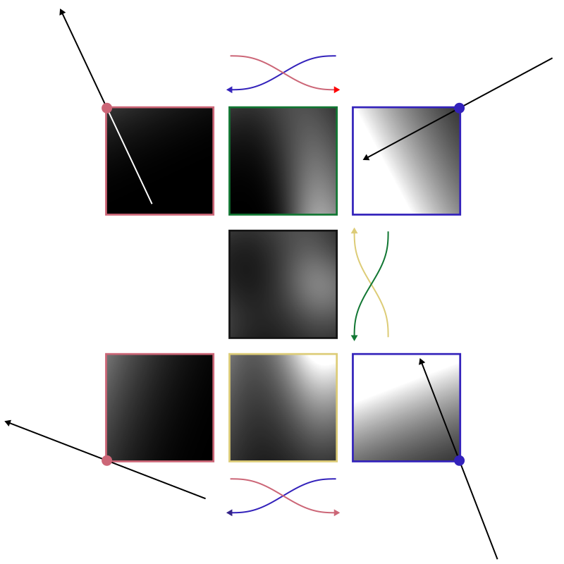
This gives us four values for p between which we now have to interpolate. We can reuse the interpolation used in the one-dimensional case by doing it in two phases: we first interpolate along the x-axis and then along the y-axis. For the x-axis we have to blend the values for v_sw and v_se, as well as the values of v_nw and v_ne. In both cases we use the distances of p to the vertices on the x-axis. Then we blend these two values using the distance of p to the northern and southern edge of the cell.

The following figure illustrates the individual steps. The images in the corners show the cell according to the four gradients. The center top image shows the cell according to v_nw and v_ne. Note how it is a blend between the top left and top right image (along the x-axis). The center bottom image shows the equivalent for v_sw and v_se. The image at the center show the final cell: a blend between the center top and center bottom image (along the y-axis).

Repeating this process for all grid cells will result in a random cloud texture similar to the one shown at the beginnin of the section. All that is missing is the additional offset we have ignored so far. But this comes down to adding a random value after evaluating the value for a given gradient. The following animation shows the entire process for a 3×3 grid:

1. Cells accoring to their south-western gradient v_sw.
2. Cells accoring to their southern gradients v_sw and v_se.
3. The fully interpolated cells.
4. Adding a random offset to each gradient.

The last steps adds a irregularity to the image that is not limited to a single cell. This way it becomes harder to spot the underlying grid:

There is only one thing left we have not covered yet but that is already used in all of the images above: we need to normalize the output of the noise function. So far the noise function maps to an unusual range that includes negative values. A more common range would be [0, 1] where zero corresponds to black and one to white.

Given that all gradients are of unit length, it is easy to calculate the extrema of the noise function. The function can reach its maximum only at the center of a cell and only if all gradient point directly at the center. In that case its value at the center is m = 0.5 · √2 + o_max where o_max denotes the maximum value we might pick as offset. It is easy to see that the minimum is -m. Thus, we need to map the output of the noise function from [-m, m] to [0, 1].

3D clouds

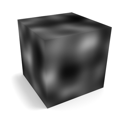
Finally we can look into generating noise volumes as shown at the very beginning of this page. Noise volumes are simply the three-dimensional equivalent of the textures we have generated in thre previous section:

And as such there is very little new about them. All we need to do is to add another dimension to the input, introduce a third phase during interpolation, and adjust the normalization.

Let’s start with the picking and the evaluation of the gradients. For a vertex v of our three-dimensional grid we now pick a three-dimensional gradient g_v = (g_x, g_y, g_z)^T. The formula to evaluate a point p is still g_v · (p - v).

In the two-dimensional case we first interpolated along the x-axis twice, and then once along the y-axis to blend between all four vertices. In the three-dimensional case we now have to interpolate between eight enclosing vertices.

The idea is to first compute the top and bottom face of the cube as described for the two-dimensional case and then interpolate between the two in a third phase (along the z-axis). Or in other words, we now interpolate along the x-axis four times, then twice along the y-axis and finaly once along the z-axis.

Finally we have to adjust the normalization of the output, since the range of our function has changed. The reason is simple: the distance between the enclosing vertices and the center of the cell is now larger. It is now half the diagonal of the unit cube instead of the unit square. This gives us a new maximum of m = 0.5 · √3 + o_max.

Implementation

If you have not already, I recommend reading the general notes on the source code and the included math package first. In particular, if you are not familiar with Java.

You can find the implementation of the gradient noise in Noise.java – a single class with less than 200 lines of code. A short example of how to generate a 2D texture as shown above is given in NoiseTexture.java.

The implementation allows to specify frequencies separately for each axis. While the function always maps from [0, 1]³ to [0, 1], we can scale the input such that it spans multiple unit sized cells. For example the texture generated in the section discussing the two-dimensional case scaled the input by a factor of three resulting in a 3×3 grid.

Noise instances are immutable, i.e., you cannot change the the random seed or the frequencies once the function is initialized. The class only has a single constructor method:

/**
 * Creates a new noise function based on the given seed and with the given
 * frequencies.
 *
 * @param seed random generator seed
 * @param fx   frequency along x-axis
 * @param fy   frequency along y-axis
 * @param fz   frequency along z-axis
 */
public Noise(long seed, float fx, float fy, float fz) {
    // Initialization code
}

Furthermore, the class provides a single public method to sample the noise volume. Except for some utility methods, all of the logic is implemented in these two methods:

/**
 * Samples the noise function at the given point.
 *
 * @param x x-coordinate in range {@code [0, 1]}
 * @param y y-coordinate in range {@code [0, 1]}
 * @param z z-coordinate in range {@code [0, 1]}
 * @return the sampled value in range {@code [0, 1]}
 */
public float sample(float x, float y, float z) {
    // Sampling code
}

Initialization

The initialization is for the most part straight-forward. We have to ensure that we pick the correct number of grid points and that the distribution of our pseudo-random gradients is not skewed.

The number of grid points can be derived from the given frequencies. For example, given the frequencies (2.2, 3.5, 1.8) we need to create a grid of size 4×5×3. However, we have to consider the literal edge case that a frequency is an integer (see the example in the comment):

// Consider the example fx = fy = fz = 1. To sample the point (1, 1, 1)
// we need to interpolate between the vertices (1, 1, 1), (2, 1, 1),
// (1, 2, 1), etc. Thus, the grid must be of size 3x3x3.
int gridX = (int) freqX + 2;
int gridY = (int) freqY + 2;
int gridZ = (int) freqZ + 2;

A naive approach to picking the gradients is to first pick a random point in the unit cube and then normalize the resulting vector. The problem with this method is that it does not result in a uniform distribution: a gradient pointing at a vertex of the cube is more likely to be picked than a gradient pointing at the center of a face. The problem and an alternative approach that guarantees a uniform distribution is discussed here. Its implementation is fairly straight-forward:

// For each vertex, pick a random point on the unit sphere and a random
// offset (intercept).
Random rng = new Random(seed);
int nVertices = gridX * gridY * gridZ;
this.gradients = new Vec3fList(nVertices);
this.offsets = new float[nVertices];
Vec3f gradient = new Vec3f();
for (int i = 0; i < nVertices; i++) {
    double theta = 2d * PI * rng.nextDouble();
    double z = 2d * rng.nextDouble() - 1d;
    double p = sqrt(1d - z * z);
    gradient.set((float) (p * cos(theta)),
            (float) (p * sin(theta)),
            (float) z);
    gradients.add(gradient);
    offsets[i] = rng.nextFloat() * (2f * OFFSET_RANGE) - OFFSET_RANGE;
}

Note how the snippet already includes picking of the random offsets.

Sampling

The sampling consist of three steps. The scaling of the input, the evaluation of and the interpolation between the eight enclosing gradients, and the normalization of the output.

Scaling the input comes down to multiplying the input with the frequencies of the noise function. Since we derive the grid indices directly from the scaled coordinates,it is important to sanitize the input here.

// Ensure bounds and map from [0, 1] to [0, frequency].
float sx = max(0f, min(x, 1f)) * freqX;
float sy = max(0f, min(y, 1f)) * freqY;
float sz = max(0f, min(z, 1f)) * freqZ;

// Local coordinates in the surrounding unit cube.
float px = sx - (int) sx;
float py = sy - (int) sy;
float pz = sz - (int) sz;

In this step we can also compute the cell-local coordinates, which are again in [0, 1]³. This allows us to think of the vertices of the cell as the vertices of the unit-cube (0, 0, 0), (1, 0, 0), …, (1, 1, 1).

The sampling is split into three phases as described in the previous section. In the first phase we evaluate all eight gradients and interpolate along the x-axis. For this we need to compute the smoothed distances to x = 0 and x = 1 (a and b):

// For each edge of the cube parallel to the x-axis, interpolate between
// samples taken at x = 0 and x = 1.
float distanceA = smooth(1f - px);
float distanceB = 1f - distanceA;

Where smooth(float) is the smoother of the two smoothstep functions:

/**
 * The smoother of the two smoothstep functions.
 *
 * @param x value in range {@code [0, 1]}
 * @return the smoothed value in range {@code [0, 1]}
 */
private static float smooth(float x) {
    return ((6f * x - 15f) * x + 10f) * x * x * x;
}

For the x-axis we have to interpolate between four pairs of gradients. The following code block looks up the gradients g_a and g_b for a = (0, 0, 0) and b = (1, 0, 0) and then evaluates the two linear functions g_a · (p - a) + o_a and g_b · (p - b) + o_b.

The helper function indexOf(float, float, float) returns the index of the gradient for the origin of the cell that encloses the given coordinates. You can read the name of the variable holding the result x00 as interpolated along the x-axis for fixed coordinates y = 0 and z = 0:

// Interpolate between (0, 0, 0) and (1, 0, 0).
int index = indexOf(sx, sy, sz);
gradients.get(index, gradient);
point.set(px, py, pz);
float a = gradient.dot(point) + offsets[index];

index = indexOf(sx + 1f, sy, sz);
gradients.get(index, gradient);
point.set(px - 1f, py, pz);
float b = gradient.dot(point) + offsets[index];

float x00 = distanceA * a + distanceB * b;

We have to do this three more times to compute x10, x01, and x11 – I won’t show this here. We can then interpolating along the y- and z-axis which is much less code:

// For each face of the cube parallel to the xy-plane, interpolate
// between the values for its two edges parallel to the x-axis.
distanceA = smooth(1f - py);
distanceB = 1f - distanceA;
float xy0 = distanceA * x00 + distanceB * x10;
float xy1 = distanceA * x01 + distanceB * x11;

// Interpolate between the values for the two faces parallel to the
// xy-axis.
distanceA = smooth(1f - pz);
distanceB = 1f - distanceA;
float xyz = distanceA * xy0 + distanceB * xy1;

Finally, we have to normalize the output which comes down to scaling it by the values described in the previous section:

// Normalize the value to [0, 1].
return xyz / (UNIT_CUBE_DIAGONAL + OFFSET_RANGE) + 0.5f;

That’s it. To get more familiar with the code I recommend looking into the example provided in NoiseTexture.java.